SPSS

One-Way

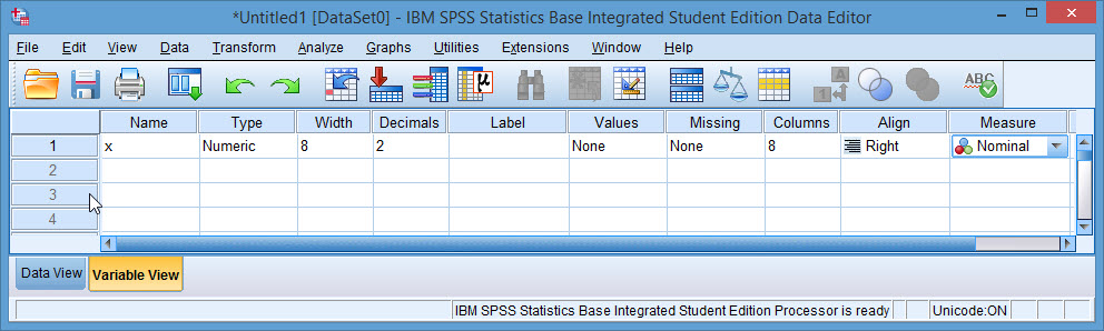
1. Once opening SPSS, click on the Variable View tab on the bottom of your SPSS window.

   

2. For a One – Way ANOVA test, you need one Numerical (Scale) variable and one Categorical (Nominal) variable defining your groups. For Example: You are measuring ACT scores (Numerical) between different high schools (Categorical). Click on cell 1, under Name, and enter the name of your first variable. Hit enter and fill in the name of your second variable.

   

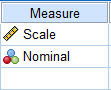
3. In column 10, under Measure, select the drop down box and choose the appropriate option for each variable. Choose Scale for your Numerical variable and Nominal for your Categorical variable.

   

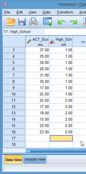
4. Click on the Data View tab on the bottom left of your SPSS window. Starting in row 1, enter all of the values of your Numerical variable, pressing enter after each new value.

5. Starting in row 1, enter all of the values of your Categorical variable, pressing enter after each new value. When entering values for a Categorical variable use numeric codes, with a different number representing each different value. For Example: In the case of gender use 0 for male and 1 for female.

   

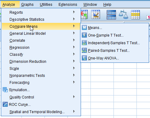
6. Once all of your data values are entered, go to the Analyze menu at the top of your SPSS window. Choose Compare Means -> One-Way ANOVA…

   

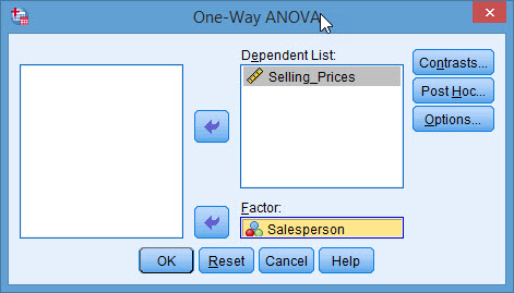
7. Choose your Numerical variable to be your Dependent variable and add it to your Dependent List. Do this by selecting the variable, in the list to the left, so it is highlighted orange, then click the square arrow button to the left of the Dependent List box.

8. Choose your Categorical as your Factor. Do this by selecting the variable, in the list to the left, so it is highlighted orange, then click the square arrow button to the left of the Factor box.

9. Click OK.

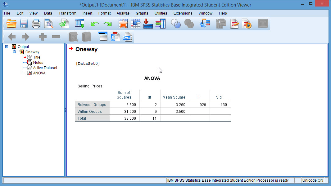
10. The output includes an ANOVA table with calculations for Sum of Squares, degrees of freedom (df), Mean Square, F Statistic, and p-value (Sig.).

    

Two-Way

1. Once opening SPSS, click on the Variable View tab on the bottom of your SPSS window.

   

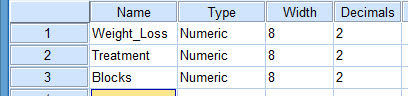
2. For a Two–Way ANOVA test, you need one Numerical (Scale) variable and two Categorical (Nominal) variables defining your groups. For Example: You are measuring ACT scores (Numerical) between different high schools (Categorical) and by Gender (Categorical). Click on cell 1, under Name, and enter the name of your first variable. Hit enter and fill in the name of your second variable. Repeat, to enter third variable.

   

3. In column 10, under Measure, select the drop down box and choose the appropriate option for each variable. Choose Scale for your Numerical variable and Nominal for your Categorical variables.

   

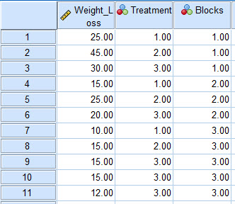
4. Click on the Data View tab on the bottom left of your SPSS window. Starting in row 1, enter all of the values of your Numerical variable, pressing enter after each new value.

5. Starting in row 1, enter all of the values of your first Categorical variable, pressing enter after each new value. When entering values for a Categorical variable use numeric codes, with a different number representing each different value. For Example: In the case of gender use 0 for male and 1 for female. Repeat this step to enter the values for your second Categorical variable.

   

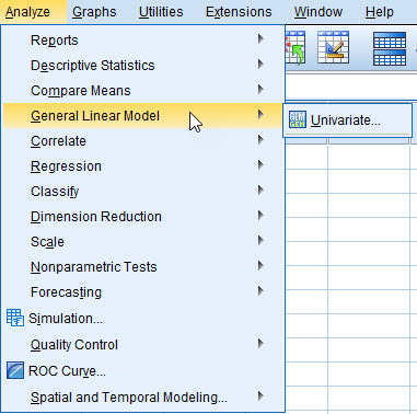
6. Once all of your data values are entered, go to the Analyze menu at the top of your SPSS window. General Linear Model -> Univariate…

   

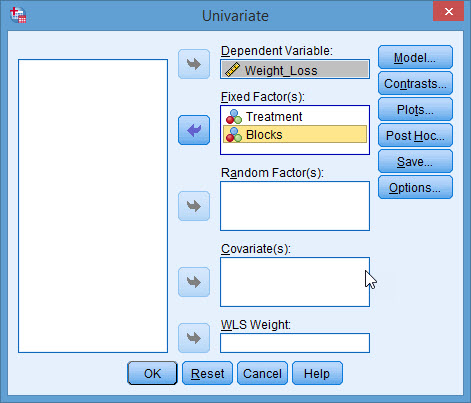
7. Choose your Numerical variable to be your Dependent Variable. Do this by selecting the variable, in the list to the left, so it is highlighted orange, then click the square arrow button to the left of the Dependent Variable box.

8. Choose your Categorical as your Fixed Factor(s). Do this by selecting one of the variables, in the list to the left, so it is highlighted orange, then click the square arrow button to the left of the Fixed Factor(s) box. Repeat this step to set your second Categorical variable as a Fixed Factor.

9. Click OK.

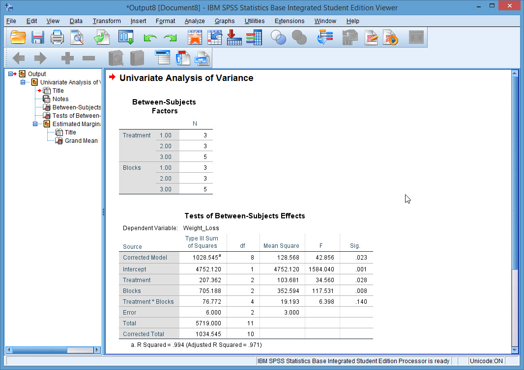
10. The first output table titled Between-Subjects Factors includes the sample size counts for each of your groups (categories).

11. The second output table titled Tests of Between-Subjects Effects is a Two - Way ANOVA table with calculations for Type III Sum of Squares, degrees of freedom (df), Mean Square, F Statistic, and p-value (Sig.). R Squared value for the calculated model is presented below the table.

    

F-Distribution

The following instructions show how to calculate a P-value given an F statistic.

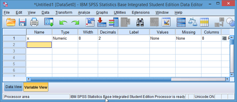
1. In order to calculate probabilities and p-values using a Distribution function you first need at least one variable defined. Once SPSS is open click on the Variable View tab at the bottom of your SPSS window.

2. Click on cell 1, under Name, and enter a name for your variable. This variable is a placeholder and will not be used in the calculations.

   

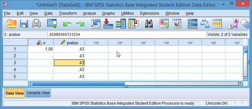
3. Click on the Data View tab at the bottom of your SPSS window. In row 1 enter a value as a placeholder. This value will not be used in the calculations.

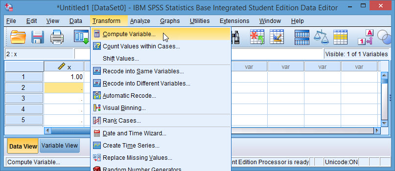
4. Click on the Transform menu at the top of your SPSS window. Choose Compute Variable…

   

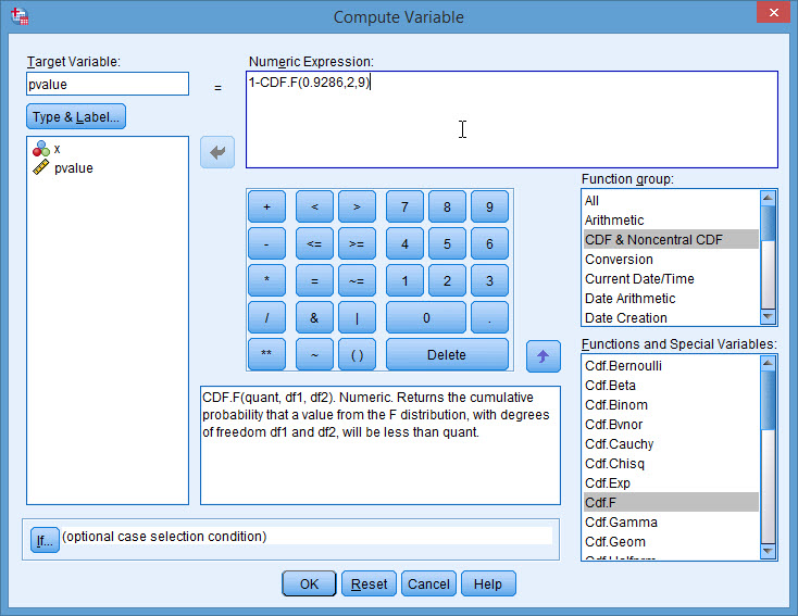
5. In the Target Variable box enter a name for your calculation. This name must be different than previously used variable names.

6. In the Function group box to the right choose CDF & Noncentral CDF.

7. In the Functions and Special Variables box in the bottom right choose Cdf.F.

8. Click on the arrow left of the Functions and Special Variables box.

9. In the Numeric Expression box at the top of your Compute Variable screen you will now see CDF(?,?,?). Using your mouse and keyboard, change the first ? into your F Statistic. Change the second ? into the degree of freedom of your numerator and the third ? into the degree of freedom of your denominator.

10. In calculating our p-value we want the probability we get a value greater than our F statistic. To do this, subtract the CDF.F function from 1 in the Numeric Expression box.

11. Click OK.

12. An output screen will pop up that can be ignored. Once you return to your Data View screen you will find that the p-value has been calculated in a column labeled after the Target Variable you chose in step 5.

    

Test for Association

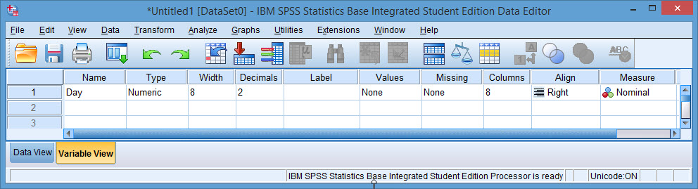
1. Once opening SPSS, click on the Variable View tab on the bottom of your SPSS window.

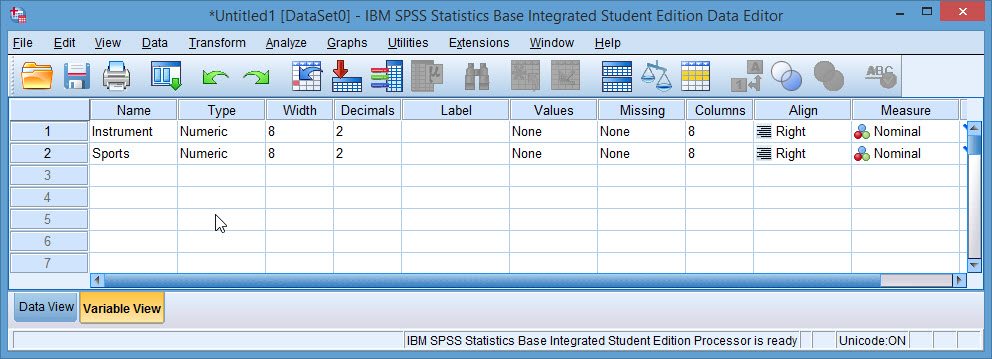
2. For a Chi - Square Test of Association, you need two Categorical (Nominal) variables. For Example: You are investigating an association between gender (Categorical) and occupation (Categorical). Click on cell 1, under Name, and enter the name of your first variable. Hit enter and fill in the name of your second variable.

3. In column 10, under Measure, select the drop down box and choose the appropriate option for each variable. Choose Nominal for your Categorical variables.

   

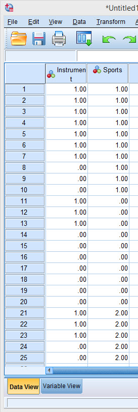
4. Click on the Data View tab on the bottom left of your SPSS window. Starting in row 1, enter all of the values of your first Categorical variable, pressing enter after each new value. When entering values for a Categorical variable use numeric codes, with a different number representing each different value. For Example: In the case of gender use 0 for male and 1 for female. Repeat this step to enter the values for your second Categorical variable.

   

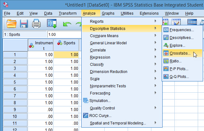
5. Once all of your data has been entered, go to the Analyze menu at the top of your SPSS window. Choose Descriptive Statistics -> Crosstabs.

   

6. Choose your first Categorical variable for your Row(s). Do this by selecting the variable, in the list to the left, so it is highlighted orange, then click the square arrow button to the left of the Row(s) box.

7. Choose your second Categorical variable for your Column(s). Do this by selecting the variable, in the list to the left, so it is highlighted orange, then click the square arrow button to the left of the Column(s) box.

   

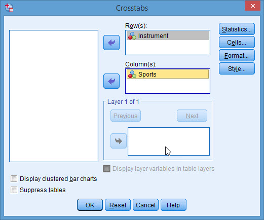
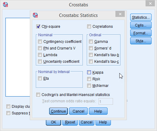
8. Click on the Statistics button, on the right of the Crosstabs Screen.

9. Check the box marked Chi-square near the top of the Crosstabs: Statistics screen, then click Continue.

10. Click OK.

    

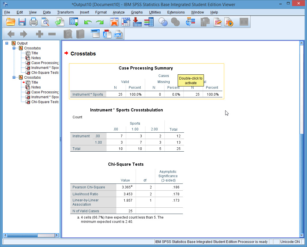
11. The output will include a Two-Way Table of your Categorical variables, titled Gender*Group Crosstabulation.

12. The Test Statistic (Value), degrees of freedom (df), and p-value (Asymptotic Significance) of your Chi-Square test for Association will be found in a table titled Chi-Square Tests, in the row labeled Pearson Chi-Square.

    

Test for Goodness of Fit

1. Once opening SPSS, click on the Variable View tab on the bottom of your SPSS window.

2. For a Chi-Square Goodness of Fit Test, you need one Categorical (Nominal) variable. Click on cell 1, under Name, and enter the name of your variable. Hit enter.

3. In column 10, under Measure, select the drop down box and choose the appropriate option for each variable. Choose Nominal for your Categorical variables.

   

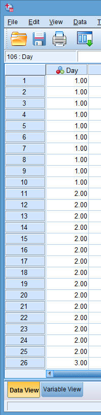
4. Click on the Data View tab on the bottom left of your SPSS window. Starting in row 1, enter all of the values of your first Categorical variable, pressing enter after each new value. When entering values for a Categorical variable use numeric codes, with a different number representing each different value. For Example: In the case of gender use 0 for male and 1 for female.

   

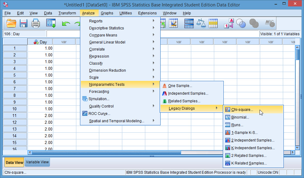
5. Once all of your data has been entered, go to the Analyze menu at the top of your SPSS window. Choose Nonparametric Tests -> Legacy Dialogs -> Chi-square…

   

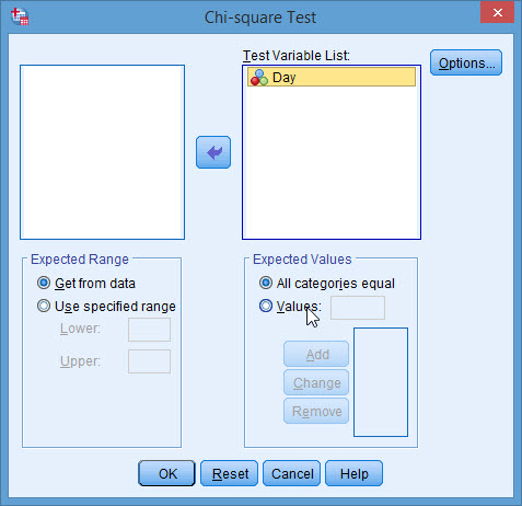
6. Choose your Categorical variable to be your Test Variable. Do this by selecting the variable, in the list to the left, so it is highlighted orange, then click the square arrow button to the left of the Test Variable List box.

7. Click OK.

   

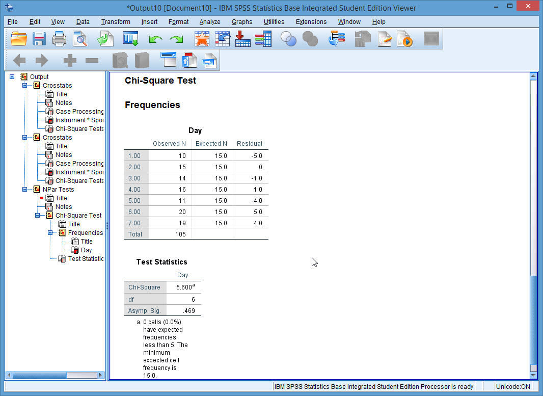
8. The results of your Chi-square Goodness of Fit test can be found in the output table titled Test Statistics. There you can find your Chi-Square statistic, degrees of freedom (df), and p-value (Asymp. Sig.).

   

Proportion

1. SPSS 24 and earlier do not come standard with a Confidence Interval for Proportions function. If you have SPSS version 18 or higher you may be able download the Confidence Interval Proportion Tool.

2. Download the Confidence Interval Proportion tool by clicking here.

3. To Install the tool, go to the Extensions menu at the top of your SPSS window. Choose Install Local Extension Bundle…

   

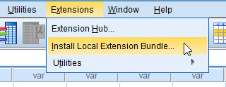
4. Find the downloaded .spe file in your Downloads folder and click Open.

   

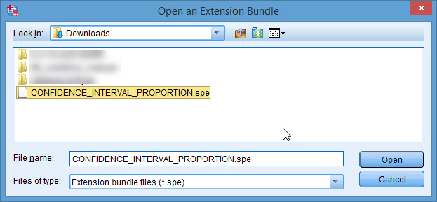
5. If any prompts pop-up click OK or Continue.

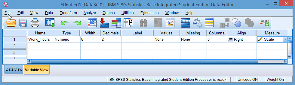
6. For a Proportions Confidence Interval, you need one Categorical (Nominal) variable with just 2 possible values. In the variable view, click on cell 1, under Name, and enter the name of your variable.

7. In column 10, under Measure, select the drop down box and choose Nominal.

   

8. Click on the Data View tab on the bottom left of your SPSS window. Starting in row 1, enter all of the values of your Categorical variable, pressing enter after each new value. When entering values for a Categorical variable use numeric codes, with a different number representing each different value. For Example: In the case of gender use 0 for male and 1 for female.

9. Once all of your data values are entered, go to the Utilities menu at the top of your SPSS window. Choose Confidence Interval Proportion.

10. First specify the test variable. Type the name of your Categorical variable in this box.

11. Ignore the box, asking you to specify a hypothesized population proportion, unless you are wanting to run a Z-Test.

12. Choose your preferred Confidence level: 95% or 99%.

13. Click OK.

14. A new data set will pop-up with multiple variables. Your z-interval for proportions can be found in columns 11 and 12 labeled lb and ub (lower bound and upper bound).

t-Interval

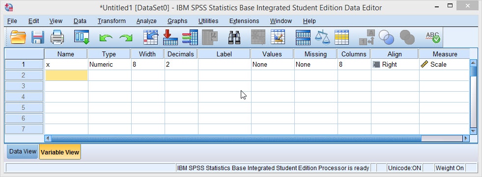
1. Once opening SPSS, click on the Variable View tab on the bottom of your SPSS window.

2. Confidence Intervals are calculated for Numerical (Scale) variables. Click on cell 1, under Name, and enter the name of your variable.

3. In column 10, under Measure, select the drop down box and choose Scale.

   

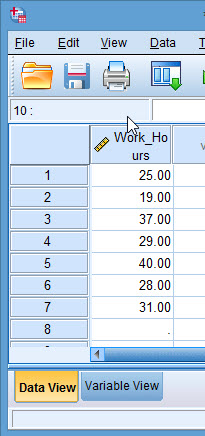
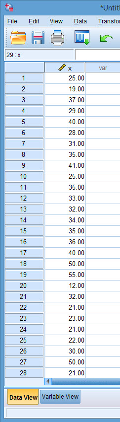
4. Click on the Data View tab on the bottom left of your SPSS window. Starting in row 1, enter all of the values of your variable, pressing Enter after each new value.

   

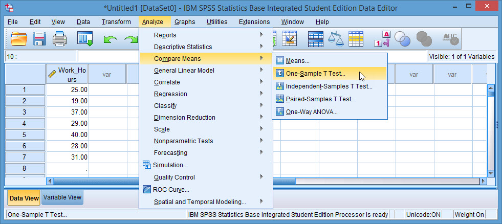
5. Once all of your data has been entered, go to the Analyze menu at the top of your SPSS window. Choose Compare Means -> One-Sample T Test…

   

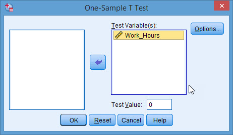
6. Choose your Numerical variable to be your Test Variable. Do this by selecting the variable, in the list to the left, so it is highlighted orange, then click the square arrow button to the left of the Test Variable(s) box.

   

7. Click on the Options… button.

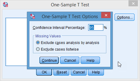
8. Set your Confidence Interval Percentage to the desired value. SPSS defaults to 95% confidence levels. Click Continue.

9. Click OK.

   

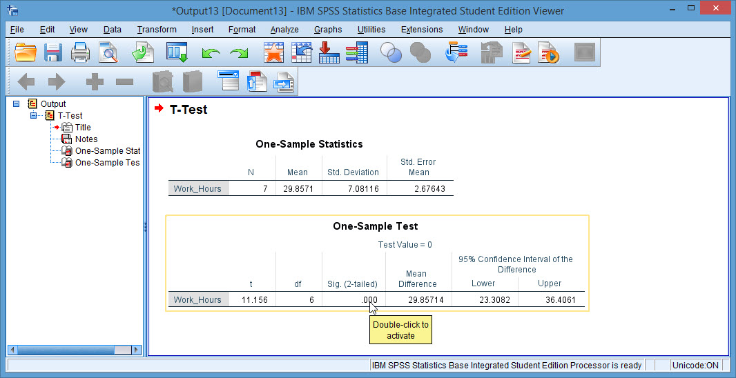
10. The results of your t-interval can be found in the output table titled One-Sample Test with your Lower and Upper bounds labeled accordingly.

    

z-Interval

1. Once opening SPSS, click on the Variable View tab on the bottom of your SPSS window.

2. Confidence Intervals are calculated for Numerical (Scale) variables. Click on cell 1, under Name, and enter the name of your variable.

3. In column 10, under Measure, select the drop down box and choose Scale.

   

4. Click on the Data View tab on the bottom left of your SPSS window. Starting in row 1, enter all of the values of your variable, pressing Enter after each new value.

   

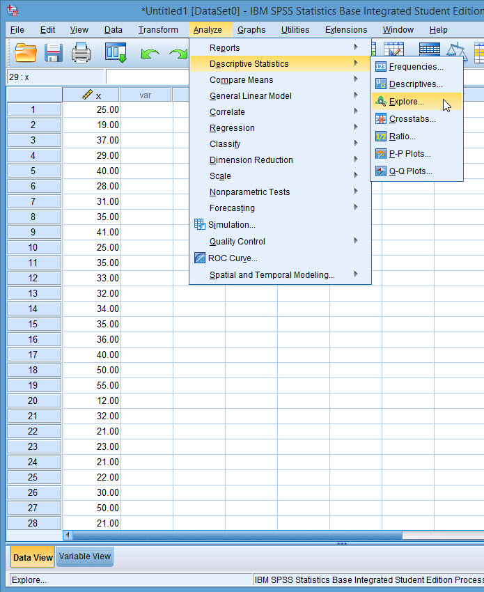
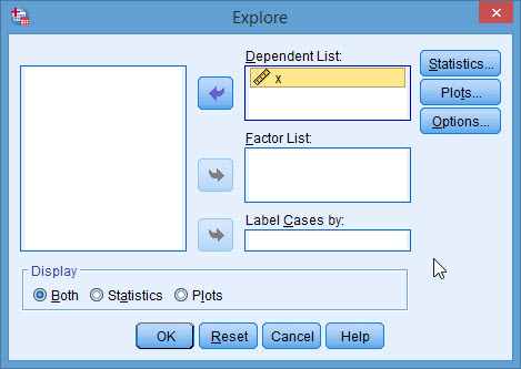
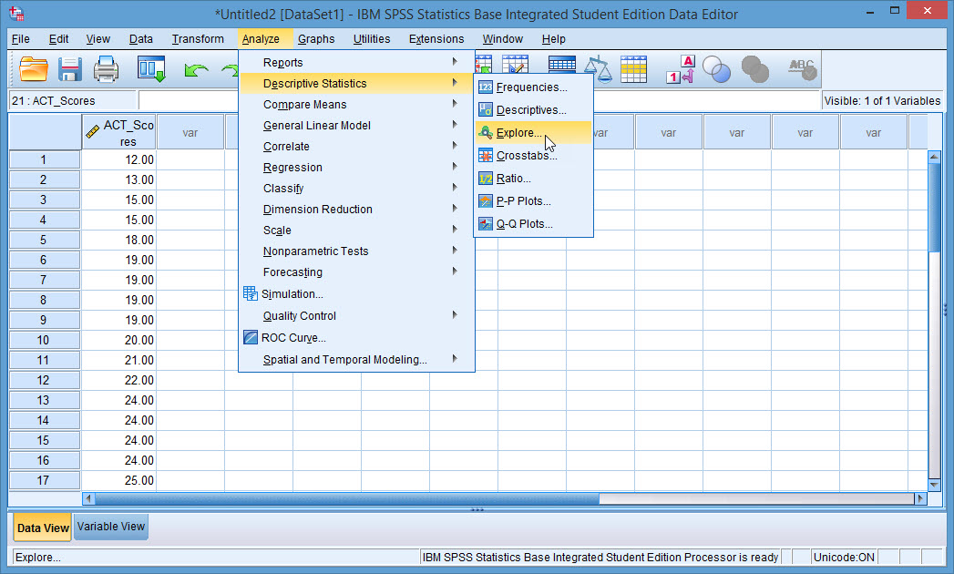
5. Once all of your data has been entered, go to the Analyze menu at the top of your SPSS window. Choose Descriptive Statistics -> Explore…

   

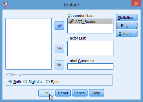
6. Choose your Numerical variable to be your Dependent Variable and add it to your Dependent List. Do this by selecting the variable, in the list to the left, so it is highlighted orange, then click the square arrow button to the left of the Dependent List box.

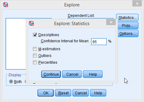
7. Click on the Statistics… button.

   

8. Make sure the Descriptives box is checked and set your Confidence Interval Percentage to the desired value. SPSS defaults to 95% confidence levels. Click Continue.

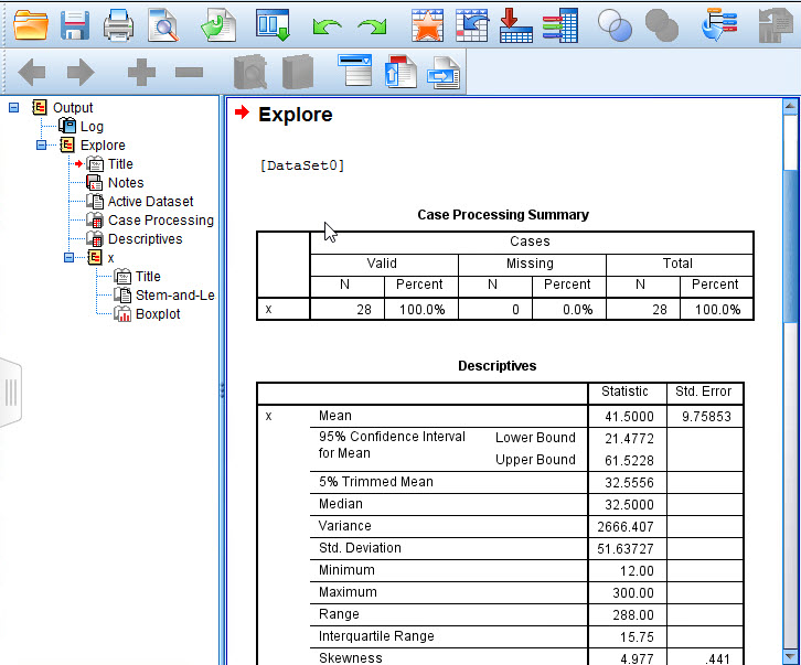
9. Click OK.

   

10. The results of your z-interval can be found in the output table titled Descriptives with your Lower and Upper bounds labeled accordingly.

    

Two Sample t-Interval

1. Once opening SPSS, click on the Variable View tab on the bottom of your SPSS window.

2. To make a Two Sample T-interval, you need one Numerical (Scale) variable and one Categorical (Nominal) variable defining your two groups. For Example: You are measuring ACT scores (Numerical) between different high schools (Categorical). Click on cell 1, under Name, and enter the name of your first variable. Hit enter and fill in the name of your second variable.

3. In column 10, under Measure, select the drop down box and choose the appropriate option for each variable. Choose Scale for your Numerical variable and Nominal for your Categorical variable.

   

4. Click on the Data View tab on the bottom left of your SPSS window. Starting in row 1, enter all of the values of your Numerical variable, pressing enter after each new value.

5. Starting in row 1, enter all of the values of your Categorical variable, pressing enter after each new value. When entering values for a Categorical variable use numeric codes, with a different number representing each different value. For Example: In the case of gender use 0 for male and 1 for female.

   

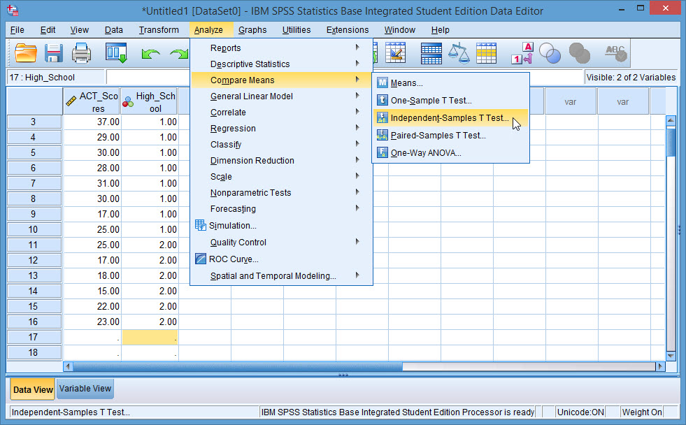
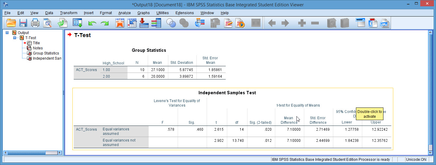
6. Once all of your data values are entered, go to the Analyze menu at the top of your SPSS window. Choose Compare Means -> Independent-Samples T Test…

   

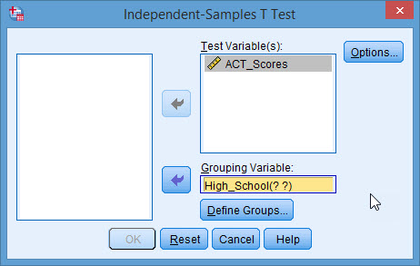
7. Choose your Numerical variable to be your Test Variable. Do this by selecting the variable, in the list to the left, so it is highlighted orange, then click the square arrow button to the left of the Test Variable(s) box.

8. Choose your Categorical variable to be your Grouping Variable. Do this by selecting the variable, in the list to the left, so it is highlighted orange, then click the square arrow button to the left of the Grouping Variable box.

   

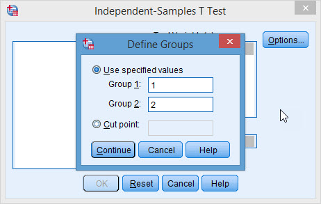
9. Click on the Define Groups… button.

10. Next to Group 1 enter the coded value you used for Group 1 in the data view screen. Next to Group 2 enter the coded value you used for Group 2 in the data view screen. Click Continue.

    

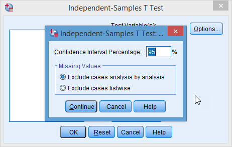
11. Click on the Options… button.

12. Set your Confidence Interval Percentage to the desired value. SPSS defaults to 95% confidence levels. Click Continue.

13. Click OK.

    

14. The results of your Two-Sample t-interval can be found in the output table titled Independent Samples Test with your Lower and Upper bounds labeled accordingly.

    

Standard Deviation

1. Once opening SPSS, click on the Variable View tab on the bottom of your SPSS window.

2. Standard Deviation is calculated for Numerical (Scale) variables. Click on cell 1, under Name, and enter the name of your variable.

3. In column 10, under Measure, select the drop down box and choose Scale.

   

4. Click on the Data View tab on the bottom left of your SPSS window. Starting in row 1, enter all of the values of your variable, pressing Enter after each new value.

   

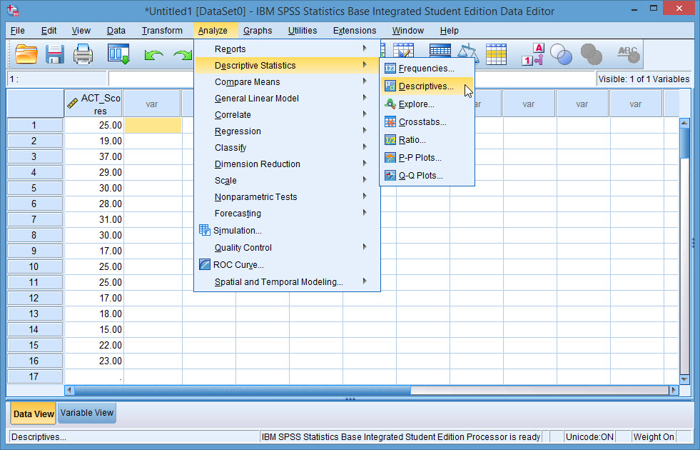
5. Once all of your data has been entered, go to the Analyze menu at the top of your SPSS window. Choose Descriptive Statistics -> Descriptives…

   

6. Choose your Numerical variable to be your Variable. Do this by selecting the variable, in the list to the left, so it is highlighted orange, then click the square arrow button to the left of the Variable(s) box.

   

7. Click on the Options… button.

8. Make sure the Std. deviation box is checked. Click Continue.

9. Click OK.

   

10. The results can be found in the output table titled Descriptive Statistics with your Std. Deviation labeled accordingly.

    

Variance

1. Once opening SPSS, click on the Variable View tab on the bottom of your SPSS window.

2. Standard Deviation is calculated for Numerical (Scale) variables. Click on cell 1, under Name, and enter the name of your variable.

3. In column 10, under Measure, select the drop down box and choose Scale.

   

4. Click on the Data View tab on the bottom left of your SPSS window. Starting in row 1, enter all of the values of your variable, pressing Enter after each new value.

   

5. Once all of your data has been entered, go to the Analyze menu at the top of your SPSS window. Choose Descriptive Statistics -> Descriptives…

   

6. Choose your Numerical variable to be your Variable. Do this by selecting the variable, in the list to the left, so it is highlighted orange, then click the square arrow button to the left of the Variable(s) box.

   

7. Click on the Options… button.

8. Make sure the Variance box is checked. Click Continue.

9. Click OK.

   

10. The results can be found in the output table titled Descriptive Statistics with your Variance labeled accordingly.

    

One Variable

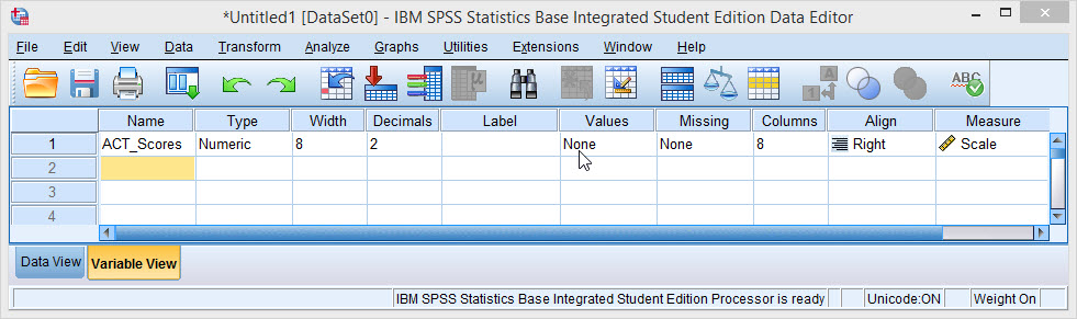
1. 1. Once opening SPSS, click on the Variable View tab on the bottom of your SPSS window.

2. The Descriptive Statistics we want to calculate are for Numerical (Scale) variables. Click on cell 1, under Name, and enter the name of your variable.

3. In column 10, under Measure, select the drop down box and choose Scale.

   

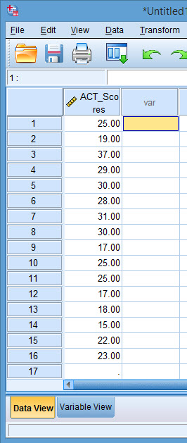
4. Click on the Data View tab on the bottom left of your SPSS window. Starting in row 1, enter all of the values of your variable, pressing Enter after each new value.

   

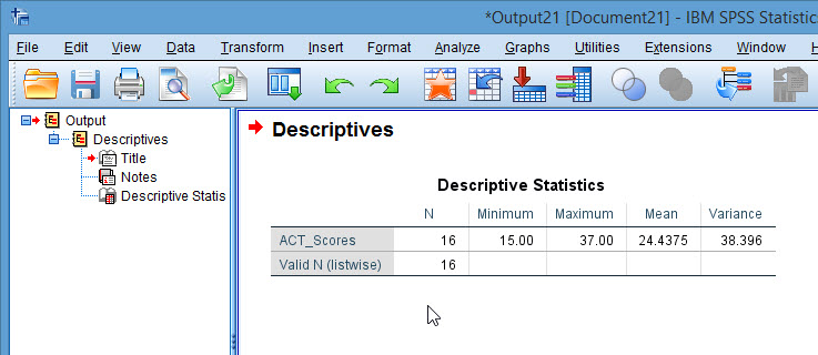
5. Once all of your data has been entered, go to the Analyze menu at the top of your SPSS window. Choose Descriptive Statistics -> Descriptives…

   

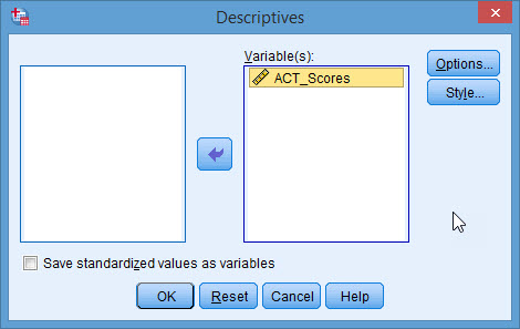
6. Choose your Numerical variable to be your Variable. Do this by selecting the variable, in the list to the left, so it is highlighted orange, then click the square arrow button to the left of the Variable(s) box.

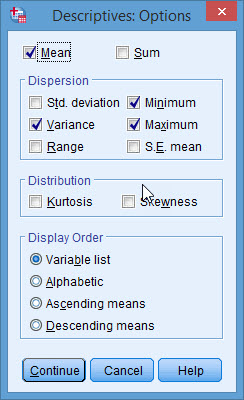
7. Click on the Options… button.

   

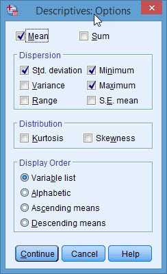
8. Now choose which Descriptive Statistics you want from your data. Your options include Mean, Sum, Std. Deviation, Variance, Range, Minimum, Maximum, S.E. mean (Standard Error), Kurtosis, and Skewness. Click Continue.

9. Click OK.

   

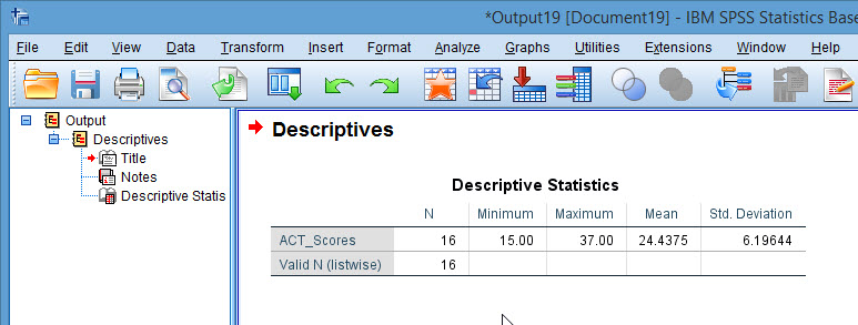
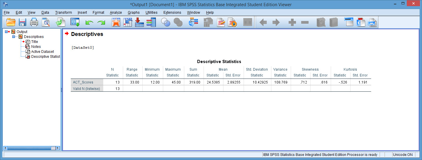
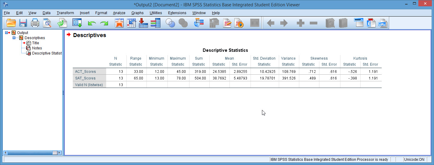
10. The results can be found in the output table titled Descriptive Statistics with your statistics labeled accordingly.

    

Two Variables

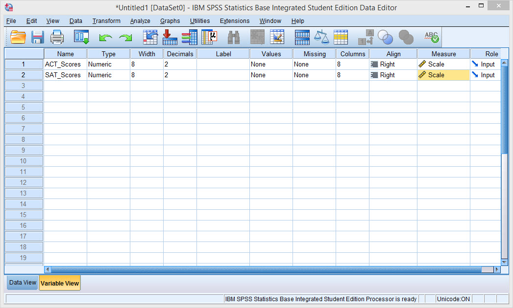
1. Once opening SPSS, click on the Variable View tab on the bottom of your SPSS window.

2. The Descriptive Statistics we want to calculate are for Numerical (Scale) variables. Click on cell 1, under Name, and enter the name of your variable. Click on cell 2 and enter the name of your second variable.

3. In column 10, under Measure, select the drop down box and choose Scale for both variables.

   

4. Click on the Data View tab on the bottom left of your SPSS window. Starting in row 1, enter all of the values of your variable, pressing Enter after each new value. Repeat for your second variable.

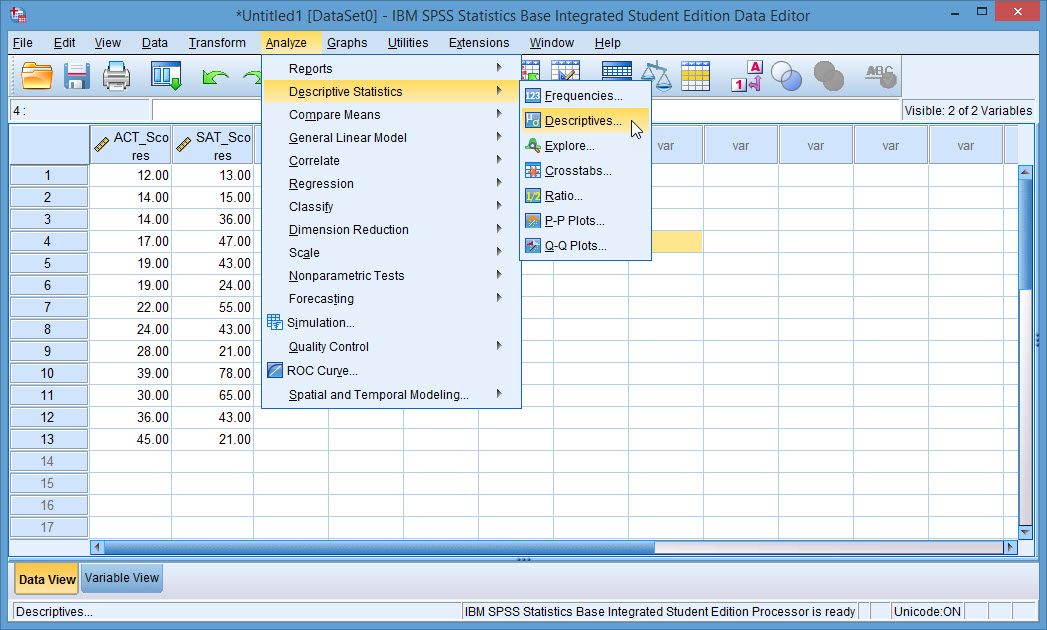
5. Once all of your data has been entered, go to the Analyze menu at the top of your SPSS window. Choose Descriptive Statistics -> Descriptives…

   

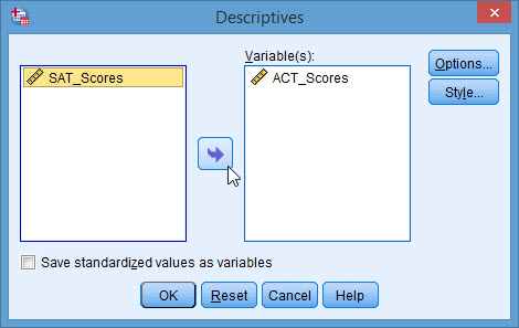
6. Choose your Numerical variables to be your Variable. Do this by selecting the variable, in the list to the left, so it is highlighted orange, then click the square arrow button to the left of the Variable(s) box. Repeat this step for your second variable.

7. Click on the Options… button.

   

8. Now choose which Descriptive Statistics you want from your data. Your options include Mean, Sum, Std. Deviation, Variance, Range, Minimum, Maximum, S.E. mean (Standard Error), Kurtosis, and Skewness. Click Continue.

9. Click OK.

   

10. The results for both variables can be found in the output table titled Descriptive Statistics with your statistics and variables labeled accordingly.

    

Bar Charts

1. Once opening SPSS, click on the Variable View tab on the bottom of your SPSS window.

2. To make a Bar Graph, you need a Categorical (Nominal) variable defining 2 or more groups. Click on cell 1, under Name, and enter the name of your first variable.

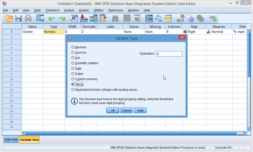
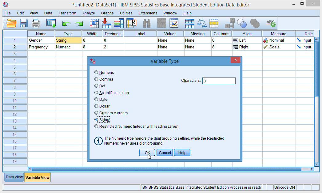
3. If you want to represent your categories in words, rather than numbers, you must change their type. In column 2, under Type, select the button on the right of the cell and check the bubble marked String.

4. Click OK.

5. In column 10, under Measure, select the drop down box and choose Nominal.

   

6. Click on the Data View tab on the bottom left of your SPSS window. Starting in row 1, enter all of the values of your variable, pressing Enter after each new value.

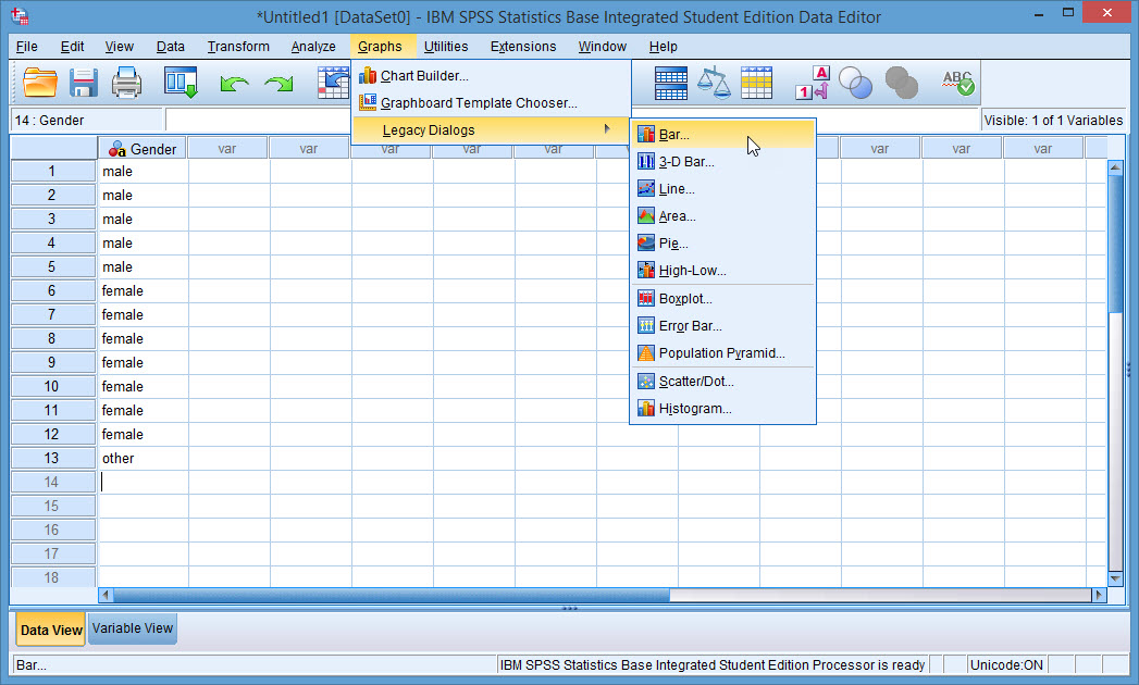
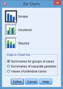
7. Once all of your data values are entered, go to the Graphs menu at the top of your SPSS window. Choose Legacy Dialogs -> Bar.

   

8. Choose the Simple option. Click Define.

   

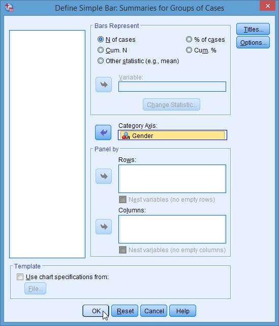
9. Choose your variable to be your Category Axis. Do this by selecting the variable, in the list to the left, so it is highlighted orange, then click the square arrow button to the left of the Category Axis box.

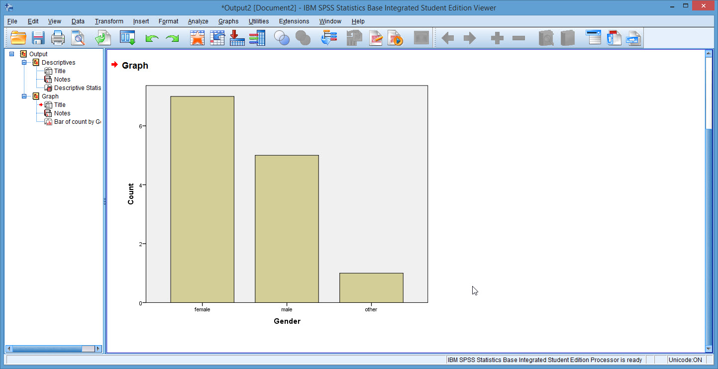
10. Click OK.

    

11. Your graph will now be included in your output screen.

    

Histogram

1. Once opening SPSS, click on the Variable View tab on the bottom of your SPSS window.

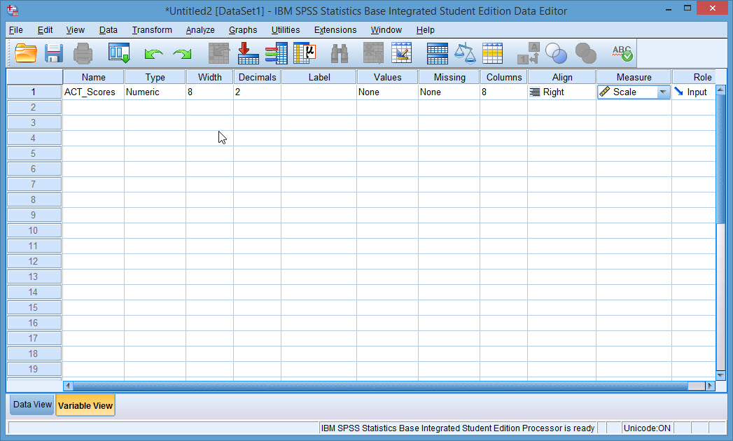
2. To make a Histogram, you need a Numerical (Scale) variable. Click on cell 1, under Name, and enter the name of your first variable.

3. In column 10, under Measure, select the drop down box and choose Scale.

   

4. Click on the Data View tab on the bottom left of your SPSS window. Starting in row 1, enter all of the values of your variable, pressing Enter after each new value.

   

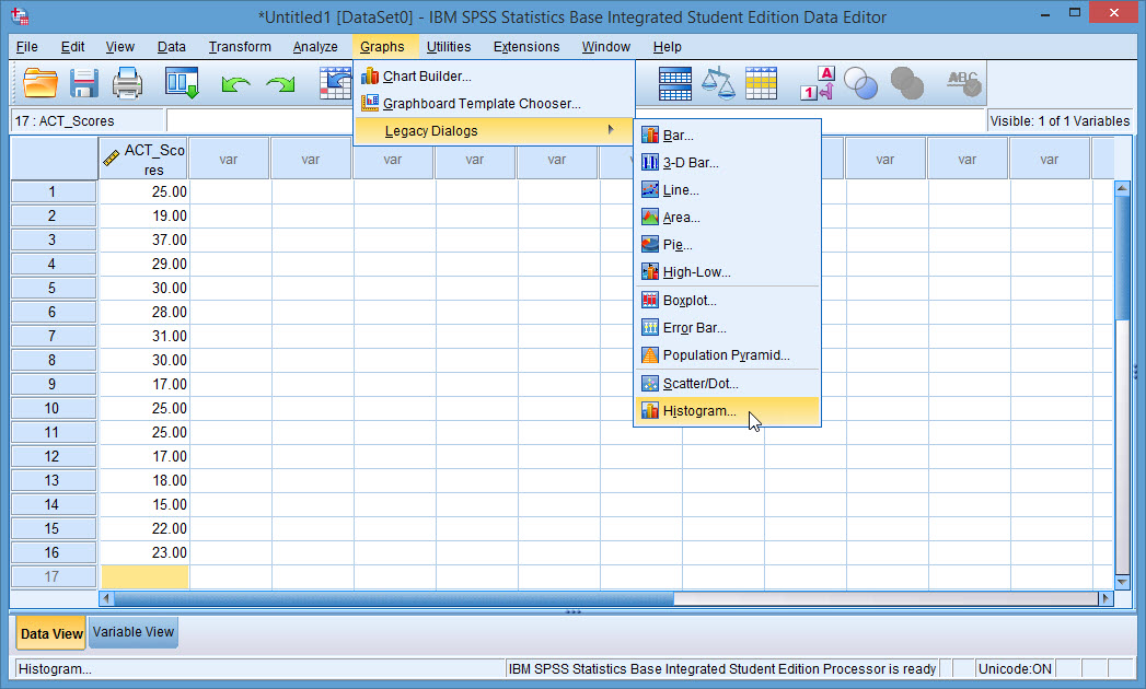
5. Once all of your data values are entered, go to the Graphs menu at the top of your SPSS window. Choose Legacy Dialogs -> Histogram.

   

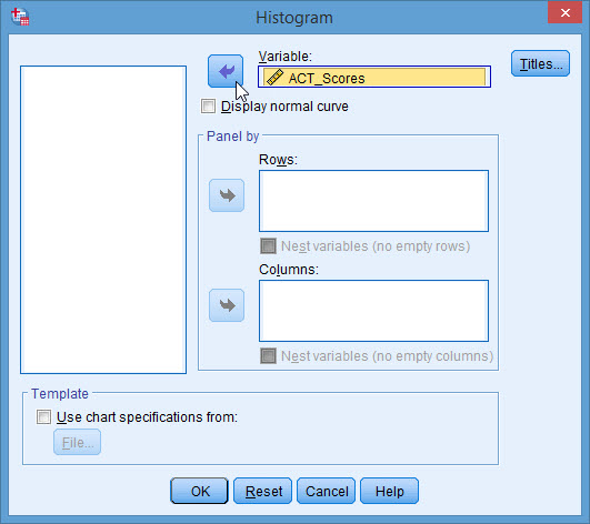
6. Choose your variable for the graph. Do this by selecting the variable, in the list to the left, so it is highlighted orange, then click the square arrow button to the left of the Variable box.

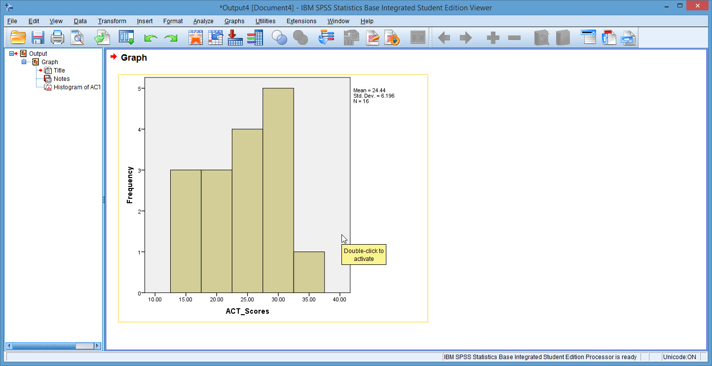
7. Click OK.

   

8. Your graph will now be included in your output screen. Mean, Std. Deviation, and Sample Size (N) are automatically presented on the top right of the Histogram.

   

Normal Probability Plot

1. Once opening SPSS, click on the Variable View tab on the bottom of your SPSS window.

2. To make a Normal Probability Plot, you need a Numerical (Scale) variable. Click on cell 1, under Name, and enter the name of your first variable.

3. In column 10, under Measure, select the drop down box and choose Scale.

   

4. Click on the Data View tab on the bottom left of your SPSS window. Starting in row 1, enter all of the values of your variable, pressing Enter after each new value.

5. Once all of your data values are entered, go to the Analyze menu at the top of your SPSS window. Descriptive Statistics -> Explore.

   

6. Choose your variable for the graph. Do this by selecting the variable, in the list to the left, so it is highlighted orange, then click the square arrow button to the left of the Dependent List box.

   

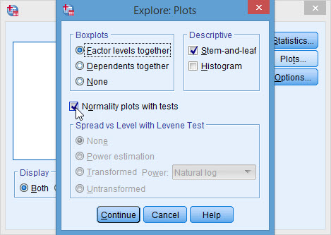
7. Click on the Plots button.

8. Make sure that the Normality plots with tests box is checked. Click Continue.

   

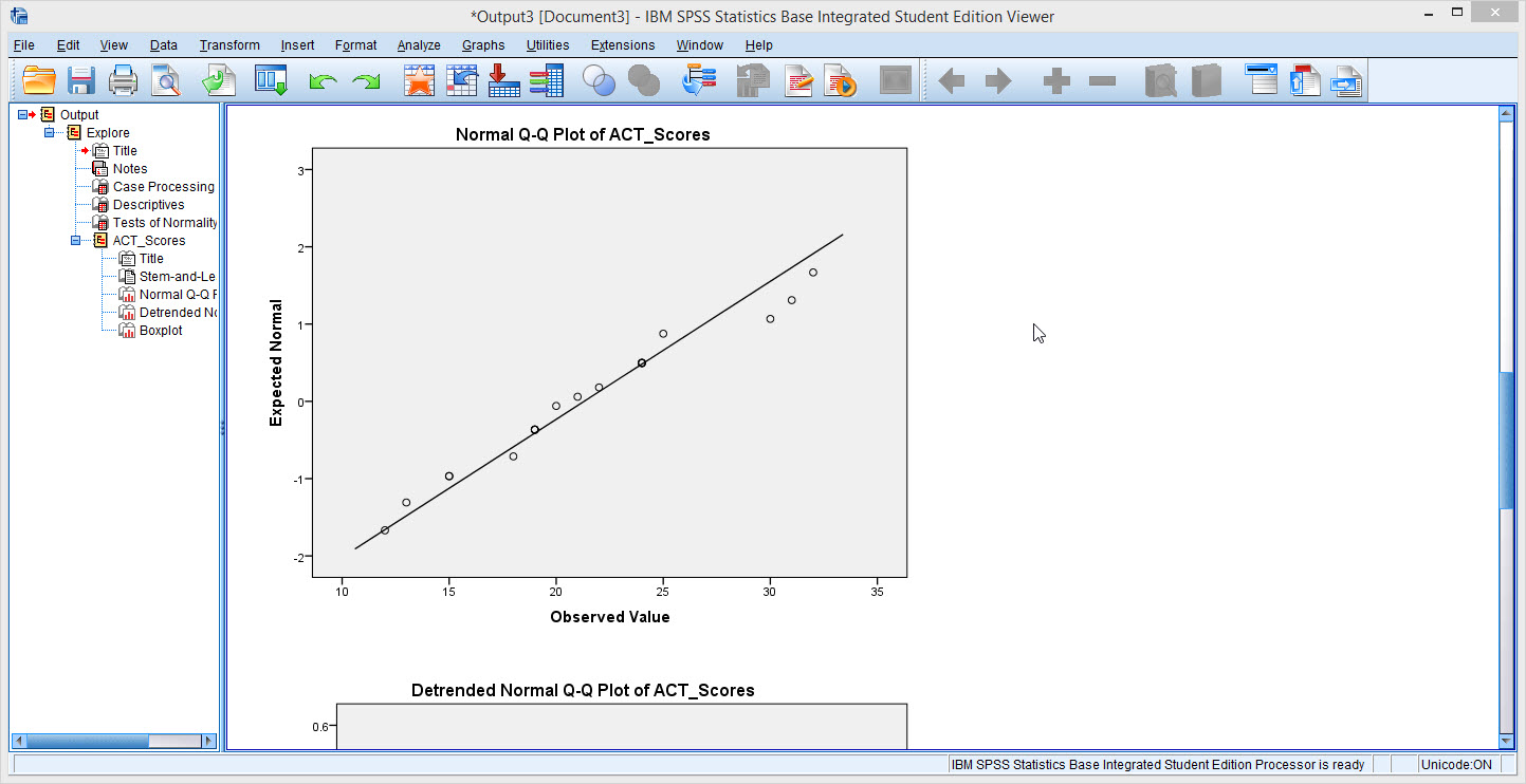
9. Click OK.

10. Your graph will now be included in your output screen labeled as Normal Q-Q Plots.

    

Pareto Chart

1. Once opening SPSS, click on the Variable View tab on the bottom of your SPSS window.

2. To make a Pareto Chart, you need a Categorical (Nominal) variable defining 2 or more groups. Click on cell 1, under Name, and enter the name of your first variable.

3. If you want to represent your categories in words, rather than numbers, you must change their type. In column 2, under Type, select the button on the right of the cell and check the bubble marked String.

4. Click OK.

5. In column 10, under Measure, select the drop down box and choose Nominal for your Categorical variable.

6. You will also need to enter a variable for the Frequency of each category.

7. In column 10 under Measure, select the drop down box and choose Scale for your Frequency variable.

   

8. Click on the Data View tab on the bottom left of your SPSS window. Starting in row 1, enter all of the categories for your Categorical variable, pressing enter after each new value. Repeat to enter the frequencies corresponding to each category.

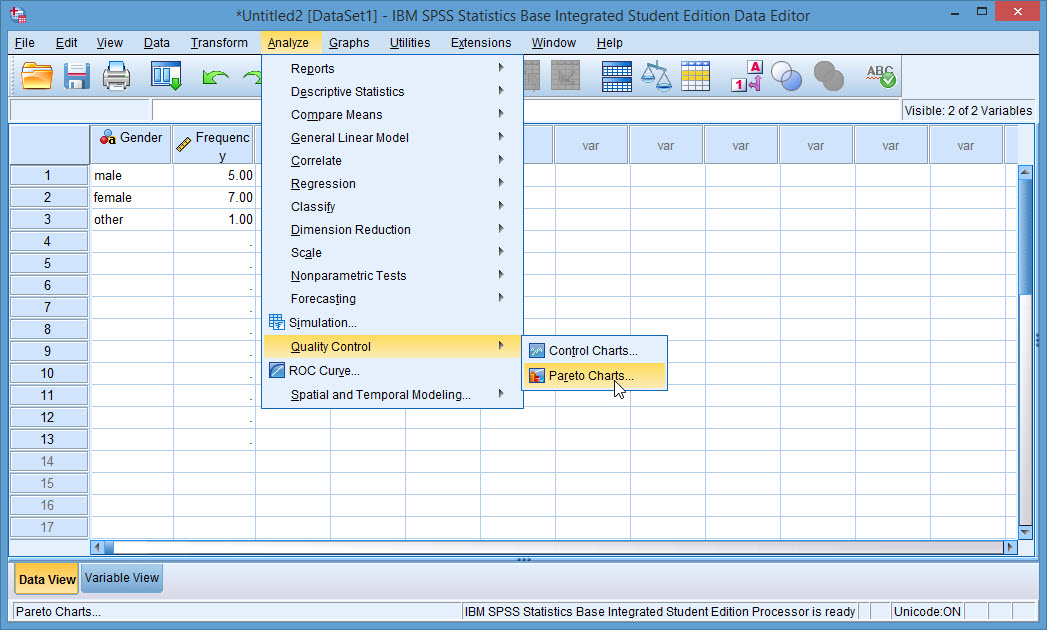
9. Once all of your data values are entered, go to the Analyze menu at the top of your SPSS window. Choose Quality Control -> Pareto Charts.

   

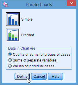
10. Choose the Simple option. Make sure that the bubble marked Counts or sums for groups of cases is checked, then click Define.

    

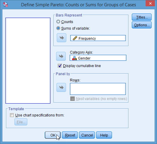
11. Choose your Categorical Variable as the Category Axis. Do this by selecting the variable, in the list to the left, so it is highlighted orange, then click the square arrow button to the left of the Category Axis box.

12. Choose your Frequencies to represent your bars. Do this by selecting the Frequency variable, in the list to the left, so it is highlighted orange, then click the square arrow button to the left of the Bars Represent box. Make sure that the bubble labeled Sums of variable is checked.

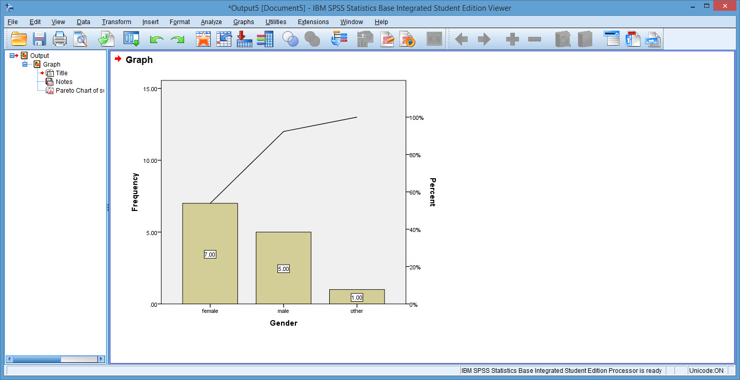
13. Click OK.

    

14. Your graph will now be included in your output screen.

    

Pie Chart

1. Once opening SPSS, click on the Variable View tab on the bottom of your SPSS window.

2. To make a Pie Chart, you need a Categorical (Nominal) variable defining 2 or more groups. Click on cell 1, under Name, and enter the name of your first variable.

3. If you want to represent your categories in words, rather than numbers, you must change their type. In column 2, under Type, select the button on the right of the cell and check the bubble marked String.

4. Click OK.

5. In column 10, under Measure, select the drop down box and choose Nominal.

   

6. Click on the Data View tab on the bottom left of your SPSS window. Starting in row 1, enter all of the values of your variable, pressing Enter after each new value.

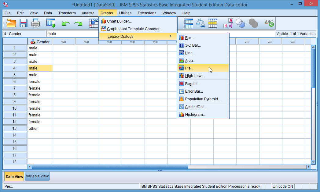
7. Once all of your data values are entered, go to the Graphs menu at the top of your SPSS window. Choose Legacy Dialogs -> Pie.

   

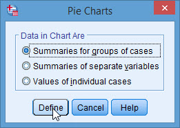
8. Click Define.

   

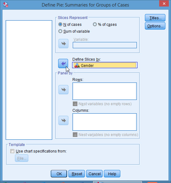
9. Choose your variable to be Defined by each Slice. Do this by selecting the variable, in the list to the left, so it is highlighted orange, then click the square arrow button to the left of the Define Slices by box.

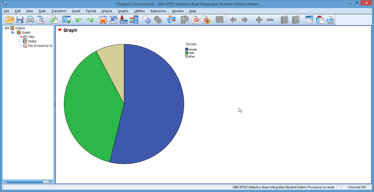
10. Click OK.

    

11. Your graph will now be included in your output screen.

    

Scatterplot

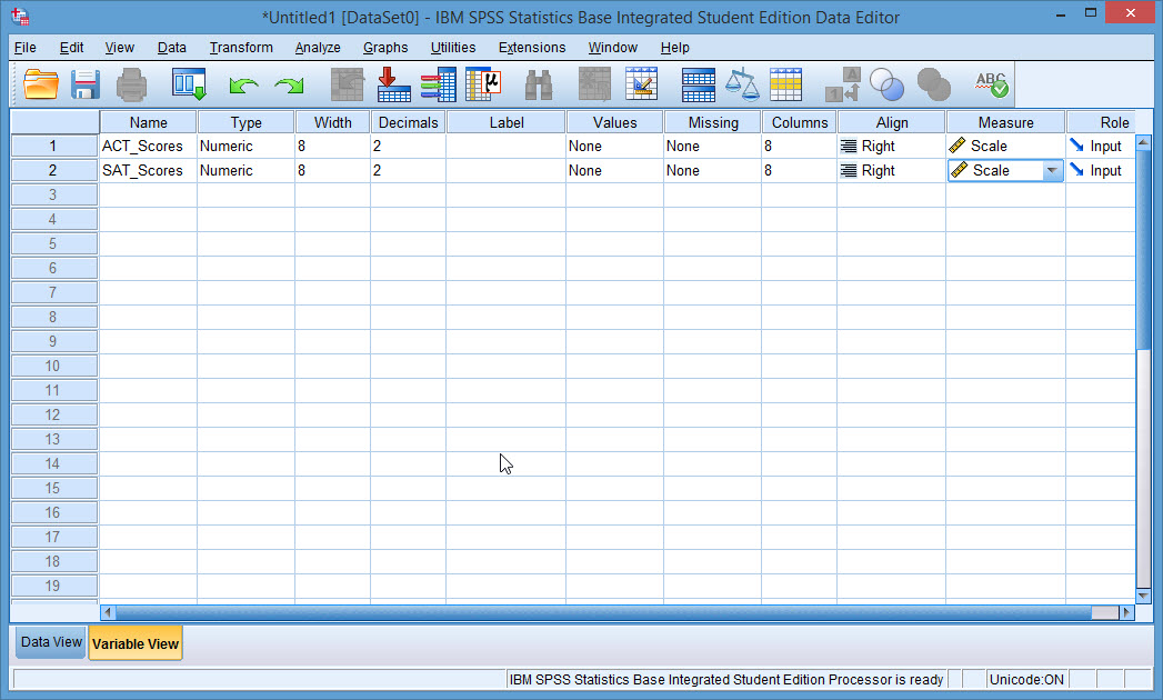
1. Once opening SPSS, click on the Variable View tab on the bottom of your SPSS window.

2. To make a Scatterplot, you need two Numerical (Scale) variables. Click on cell 1, under Name, and enter the name of your first variable. Repeat to enter name of variable 2.

3. In column 10, under Measure, select the drop down box and choose Scale. Repeat for variable number 2.

   

4. Click on the Data View tab on the bottom left of your SPSS window. Starting in row 1, enter all of the values of your variable, pressing Enter after each new value. Repeat your data entry for variable number 2. Note that in order to make a scatterplot both of your variables must be paired and have the same number of values.

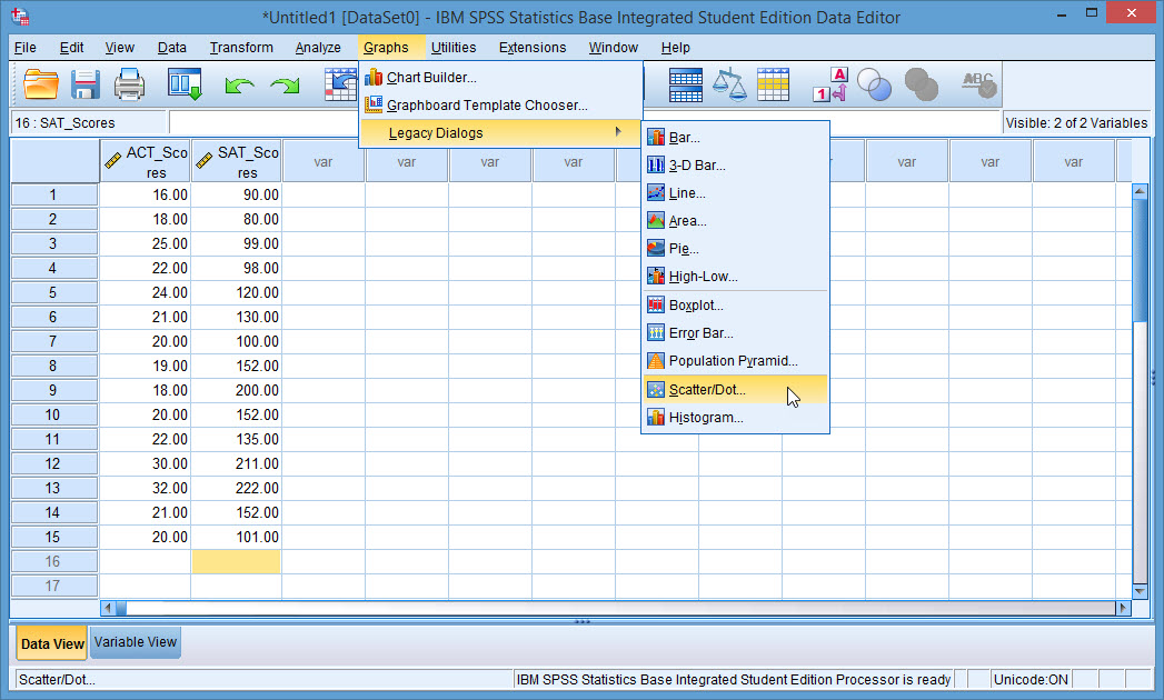
5. Once all of your data values are entered, go to the Graphs menu at the top of your SPSS window. Choose Legacy Dialogs -> Scatter/Dot.

   

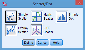
6. Choose Simple Scatter option. Click Define.

   

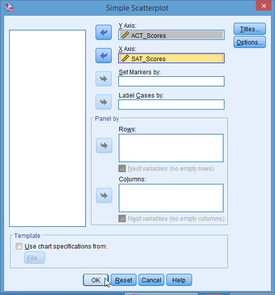
7. Choose your Dependent variable to be your Y Axis. Do this by selecting the variable, in the list to the left, so it is highlighted orange, then click the square arrow button to the left of the Y Axis box.

8. Choose your Independent variable to be your X Axis. Do this by selecting the variable, in the list to the left, so it is highlighted orange, then click the square arrow button to the left of the X Axis box.

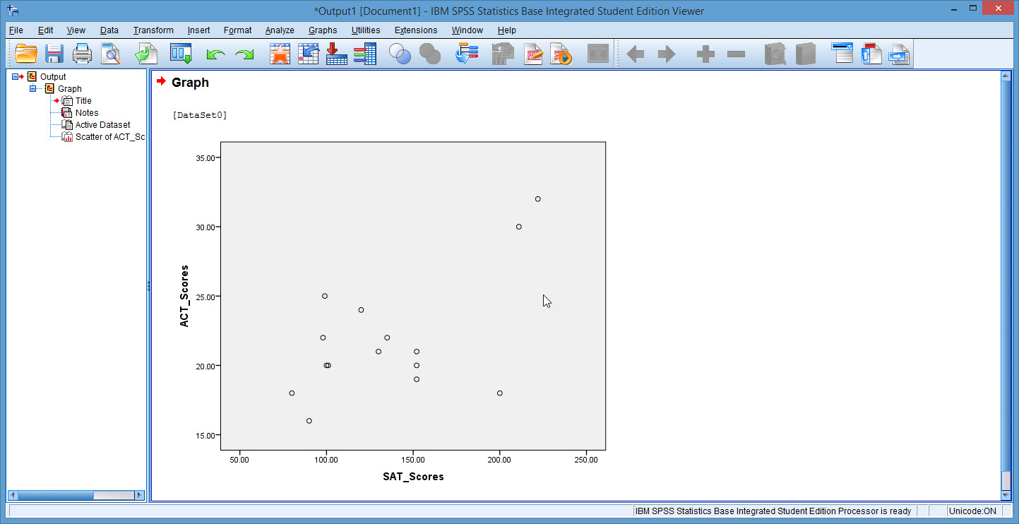
9. Click OK.

   

10. Your graph will now be included in your output screen.

    

Stem and Leaf Plot

1. Once opening SPSS, click on the Variable View tab on the bottom of your SPSS window.

2. To make a Stem and Leaf Plot, you need a Numerical (Scale) variable. Click on cell 1, under Name, and enter the name of your first variable.

3. In column 10, under Measure, select the drop down box and choose Scale.

   

4. Click on the Data View tab on the bottom left of your SPSS window. Starting in row 1, enter all of the values of your variable, pressing Enter after each new value.

5. Once all of your data values are entered, go to the Analyze menu at the top of your SPSS window. Descriptive Statistics -> Explore.

   

6. Choose your variable for the graph. Do this by selecting the variable, in the list to the left, so it is highlighted orange, then click the square arrow button to the left of the Dependent List box.

7. Click OK.

   

8. Your graph will now be included in your output screen labeled accordingly.

   

Dot Plot

1. Once opening SPSS, click on the Variable View tab on the bottom of your SPSS window.

2. To make a Dot Plot, you need a Numerical (Scale) variable. Click on cell 1, under Name, and enter the name of your first variable.

3. In column 10, under Measure, select the drop down box and choose Scale.

   

4. Click on the Data View tab on the bottom left of your SPSS window. Starting in row 1, enter all of the values of your variable, pressing Enter after each new value.

   

5. Once all of your data values are entered, go to the Graphs menu at the top of your SPSS window. Choose Legacy Dialogs -> Scatter/Dot.

   

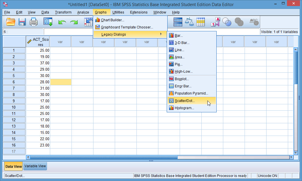
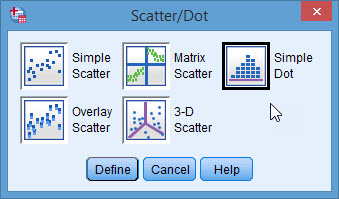
6. Choose Simple Dot option. Click Define.

   

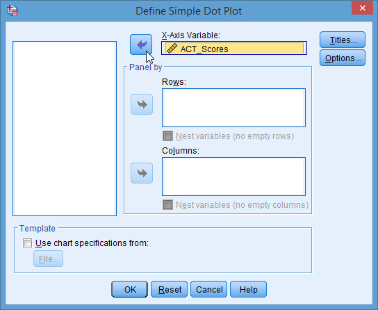
7. Choose your variable to be your X Axis. Do this by selecting the variable, in the list to the left, so it is highlighted orange, then click the square arrow button to the left of the X Axis Variable box.

8. Click OK.

   

9. Your graph will now be included in your output screen.

   

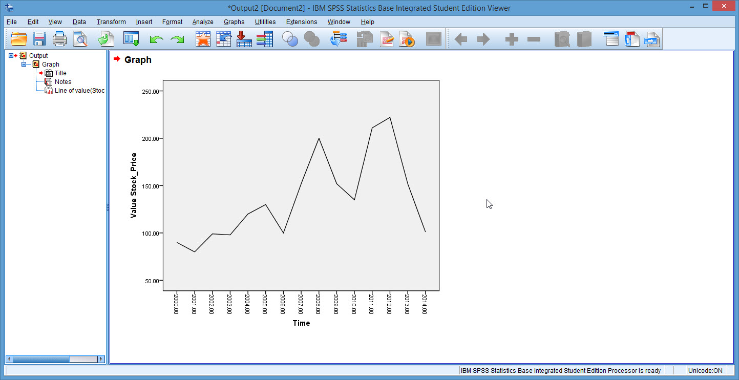
Line Graph

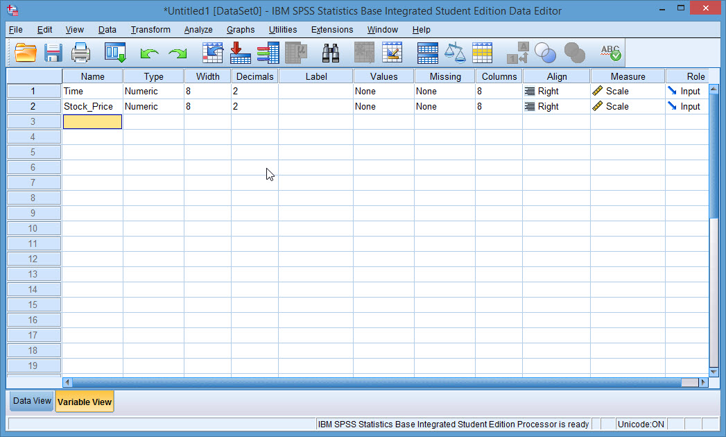
1. Once opening SPSS, click on the Variable View tab on the bottom of your SPSS window.

2. To make a Line Graph, you need two Numerical (Scale) variables. One of them is often Time. Click on cell 1, under Name, and enter the name of your first variable. Repeat to enter name of variable 2.

3. In column 10, under Measure, select the drop down box and choose Scale. Repeat for variable number 2.

   

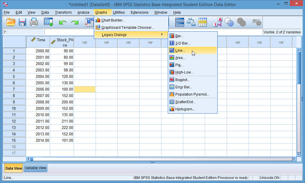
4. Click on the Data View tab on the bottom left of your SPSS window. Starting in row 1, enter all of the values of your variable, pressing Enter after each new value. Repeat your data entry for variable number 2. Note that in order to make a Line Graph both of your variables must be paired and have the same number of values.

5. Once all of your data values are entered, go to the Graphs menu at the top of your SPSS window. Choose Legacy Dialogs -> Line.

   

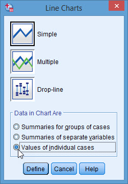
6. Choose Simple option.

7. Select the bubble labeled Values of Individual Cases. Click Define.

   

8. Choose your Dependent variable to shape your line. Do this by selecting the variable, in the list to the left, so it is highlighted orange, then click the square arrow button to the left of the Line Represents box.

9. Choose your Independent variable to be your X Axis. This is usually time. Select the Category Labels bubble Variable. Then select your independent variable, in the list to the left, so it is highlighted orange, then click the square arrow button to the left of the Variable box.

10. Click OK.

    

11. Your graph will now be included in your output screen.

    

Simple Linear Regression

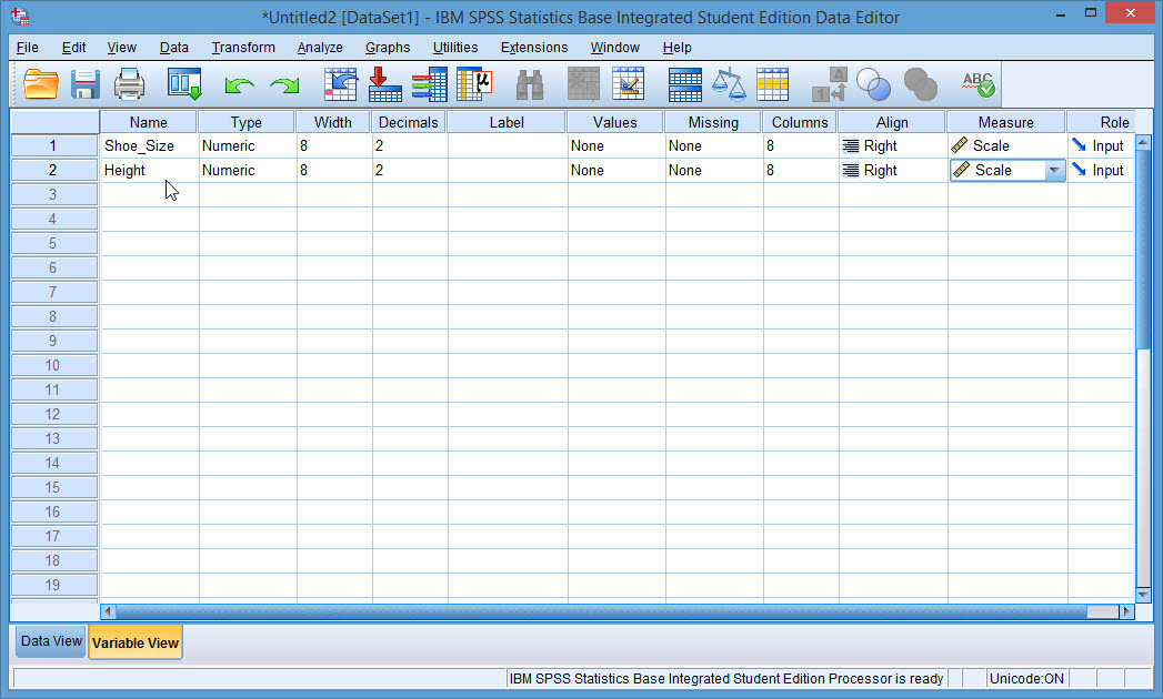
1. Once opening SPSS, click on the Variable View tab on the bottom of your SPSS window.

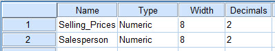
2. To perform Simple Linear Regression, you need two Numerical (Scale) variables. Click on cell 1, under Name, and enter the name of your first variable. Repeat to enter name of variable 2.

3. In column 10, under Measure, select the drop down box and choose Scale. Repeat for variable number 2.

   

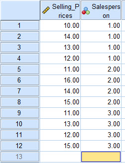
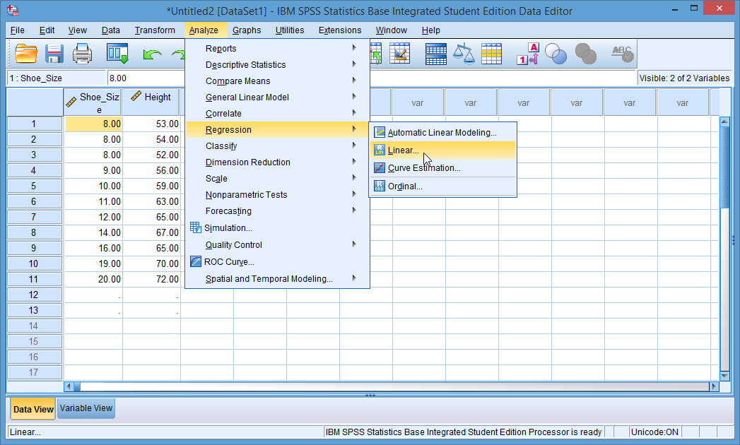
4. Click on the Data View tab on the bottom left of your SPSS window. Starting in row 1, enter all of the values of your variable, pressing Enter after each new value. Repeat your data entry for variable number 2. Note that in order to make a scatterplot both of your variables must be paired and have the same number of values.

5. Once all of your data values are entered, go to the Analyze menu at the top of your SPSS window. Choose Regression -> Linear.

   

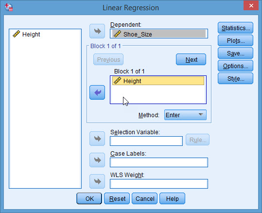
6. Choose your Dependent variable. Do this by selecting the variable, in the list to the left, so it is highlighted orange, then click the square arrow button to the left of the Dependent box.

7. Choose your Independent variable. Do this by selecting the variable, in the list to the left, so it is highlighted orange, then click the square arrow button to the left of the Block 1 of 1 box.

8. Click OK.

   

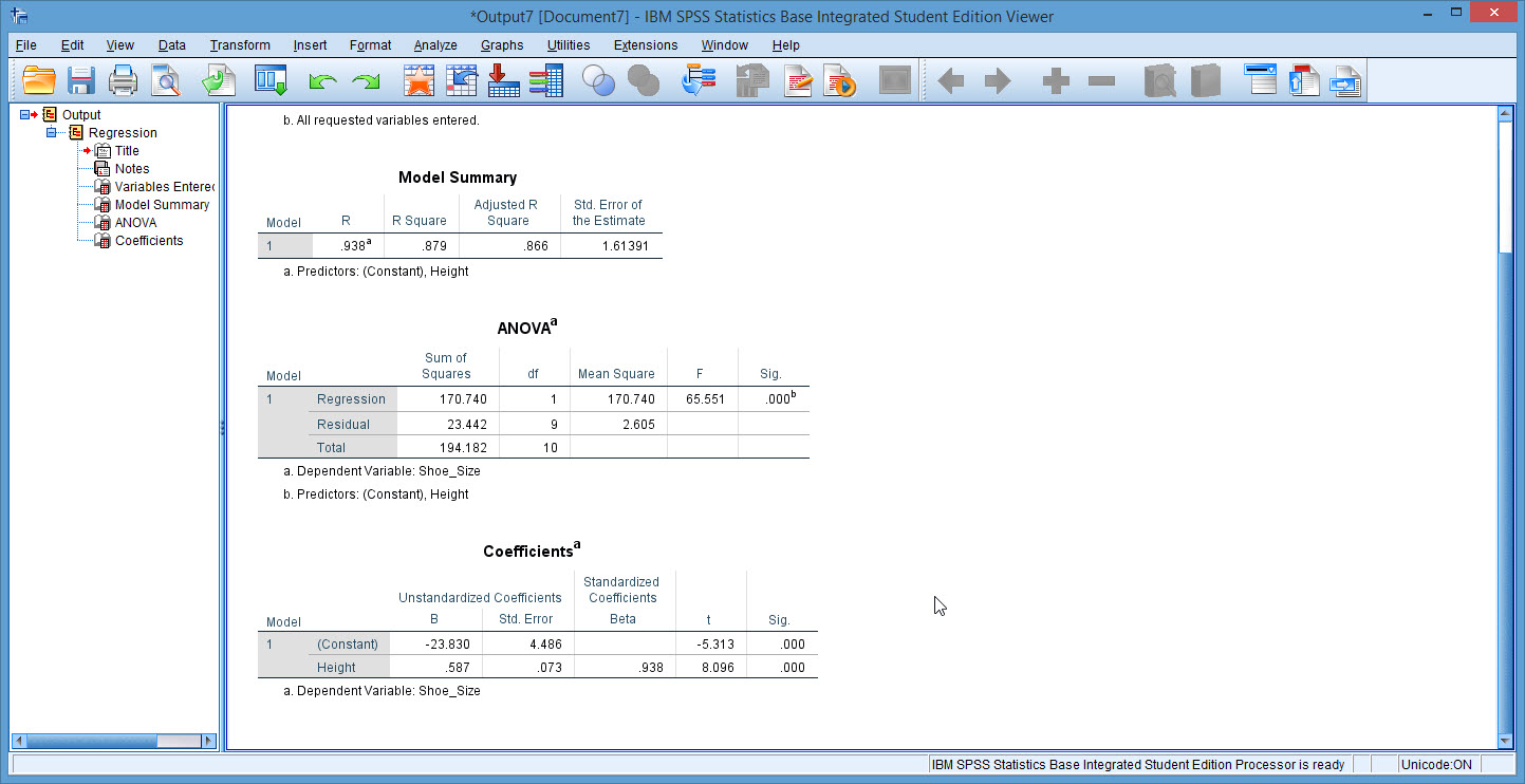
9. Your Regression output will now be included in your output screen. You can find your regression coefficients in the table labeled Coefficients.

   

Random Samples

1. Once opening SPSS, click on the Variable View tab on the bottom of your SPSS window.

2. Click on cell 1, under Name, and enter the name of your variable.

   

3. Click on the Data View tab on the bottom left of your SPSS window. Starting in row 1, enter all of the values of your variable, pressing Enter after each new value.

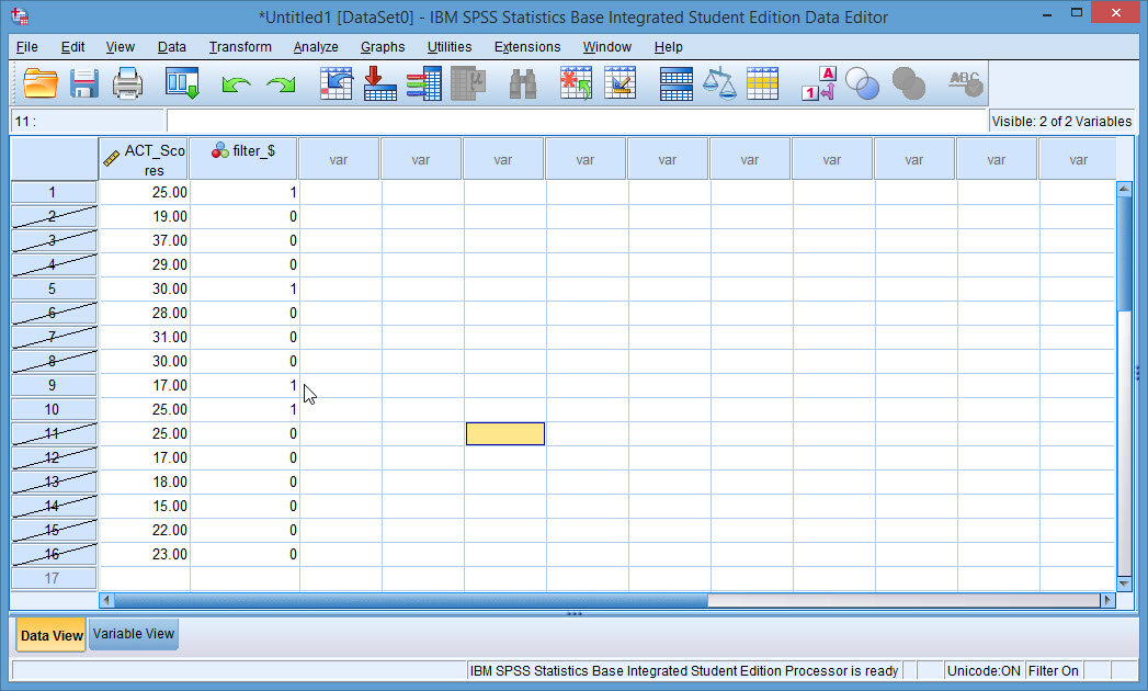
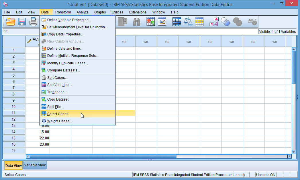
4. Once all of your data has been entered, go to the Data menu at the top of your SPSS window. Choose Select Cases.

   

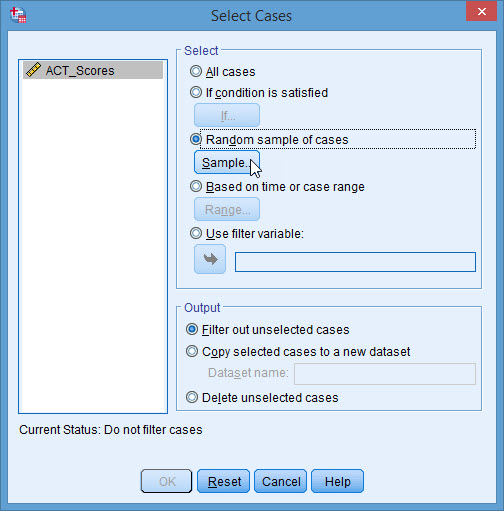
5. Select the bubble marked Random Sample of cases.

6. Click the Sample button.

   

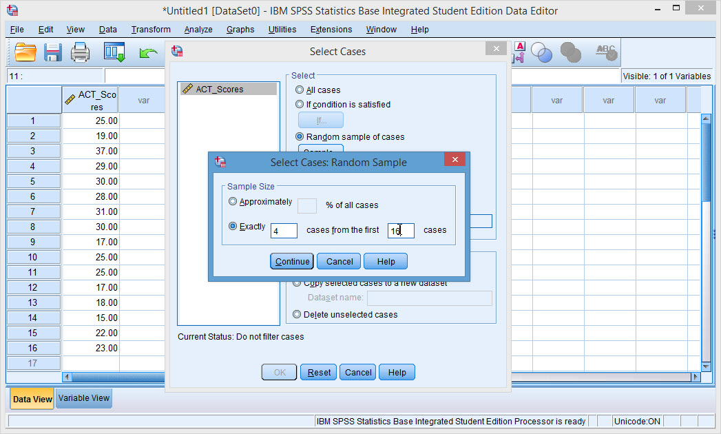
7. Either choose an approximate percentage of the population you would like sampled OR select the exact number of units you would like in your sample.

8. Click Continue.

9. Click OK.

   

10. SPSS has now chosen your sample. Values not in the sample still appear, but are seen as crossed out in the column to their left.